[.green-span]How to build and deploy probability of default models[.green-span]

Probability of default models estimate how likely a borrower is to miss payments, usually over a 12-month window. They turn credit and business data into a score that drives approve, decline, and pricing decisions. Build one well and you underwrite faster, price risk accurately, and reserve the right capital.
This guide covers what these models do, how to build and deploy one step by step, and the practices that keep them accurate and compliant. It is written for risk, lending, and product teams at banks, fintech lenders, and brands that embed small business financing.
What probability of default models do for lenders
A probability of default (PD) model outputs a score between 0 and 1 for each borrower. That score feeds the expected credit loss a lender reserves against.
Regulators and risk teams rely on this output. Per DataRobot's credit risk documentation, expected credit loss is commonly calculated as PD multiplied by loss given default and exposure at default. The same guidance notes the default target is normally defined as 90 days delinquency.
Demand for PD models is rising as lending moves into software. Embedded finance pushes credit decisions into checkout flows and dashboards, where borrowers expect answers in minutes. A reliable PD score is what lets you automate those approvals safely.
Accurate PD scores support three decisions:
- Approve or decline: rank applicants and set a cutoff that balances approvals against expected losses.
- Price and structure: match rate, term, and limit to each borrower's risk.
- Reserve capital: size loss estimates so you hold enough buffer for downturns.
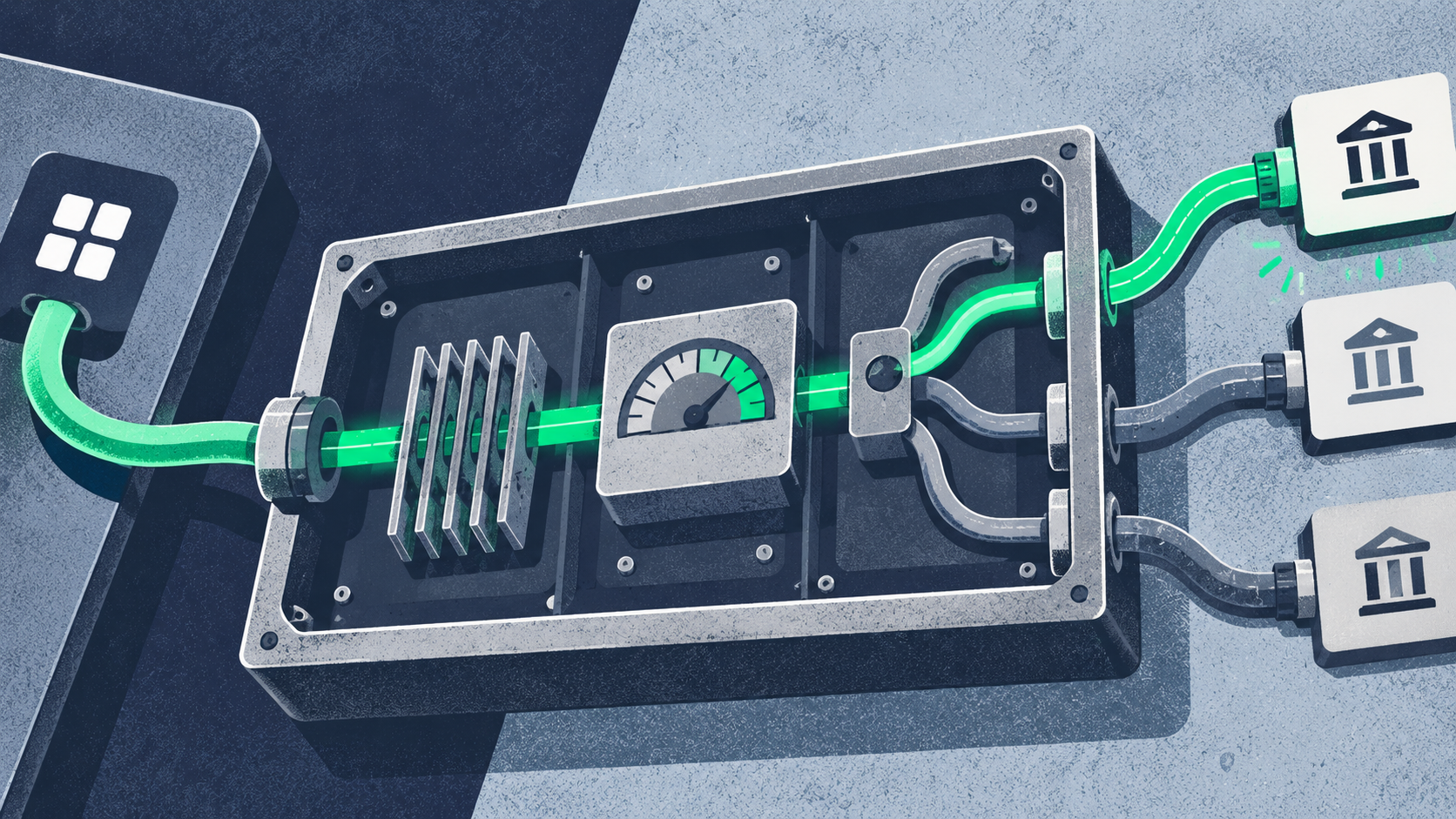
PD models are only as strong as the data behind them. Lendflow Connect aggregates banking, business, and credit data through one integration across 75+ lenders, so models score on live signals, not stale documents.
How to build and deploy a PD model step by step
Work through a disciplined lifecycle. The Federal Reserve and OCC guidance SR 11-7 spans model development, implementation, validation, and governance across the full model lifecycle.
- Define the default target. Set a clear default definition, such as 90 days past due, and the outcome window, usually 12 months.
- Assemble the data. Pull bank transactions, credit files, accounting records, and business data into one clean, labeled dataset.
- Engineer features. Build predictive variables like debt-to-income, cash-flow coverage, and delinquency history.
- Train and compare models. Test logistic regression against gradient-boosted trees such as XGBoost, then keep the best performer.
- Calibrate the scores. Convert raw outputs into true probabilities so PD feeds expected loss correctly.
- Validate independently. Have a separate team challenge the assumptions, data, and results before launch.
- Deploy into the workflow. Serve scores through an API at the point of decision, not in a spreadsheet.
- Monitor and retrain. Track score drift and realized defaults, then refresh the model on a set cadence.
Lendflow Automate turns steps 7 and 8 into production infrastructure. Its Trust Score agent returns an explainable composite risk score, and its agents deliver up to 80% faster document review and 65% faster time-to-decision.
Best practices for accurate, compliant PD models
Strong PD programs win on data quality and governance, not model complexity. Lendflow Intelligence customers report 85% faster time-to-decision and a 60% lift in application conversion by automating the pipeline around complete data.
- Evaluate with the right metrics. Judge PD models with AUC, the Gini coefficient, and the KS statistic, not raw accuracy.
- Convert AUC to Gini. The Gini coefficient equals 2 times AUROC minus 1, a standard credit-scoring measure.
- Target a defensible KS. Analysts often treat a KS between 0.3 and 0.7 as acceptable; very high values can signal overfitting.
- Keep validation independent. SR 11-7 treats effective challenge as the guiding principle of model risk management.
- Explain every score. Use methods like SHAP so you can tell an applicant why a decision happened.
- Watch for drift. Monitor score distribution and realized defaults so you catch deterioration early.
Probability of default models are core infrastructure for modern lending. Build them on a disciplined lifecycle: define the target, engineer features, validate independently, deploy through an API, and monitor for drift. Anchor the whole pipeline on complete, real-time data, because model quality follows data quality.
Lendflow connects the data, decisioning, and automation layers so your PD models move from spreadsheets into production. When you are ready to connect capital and grow, book a demo or talk to our team.
Frequently asked questions
What is a probability of default model?
It is a statistical or machine learning model that estimates the likelihood a borrower defaults within a set window, usually 12 months.
What data do PD models need?
They use bank transactions, credit bureau data, accounting records, and business attributes. Cleaner, fresher, and more complete data produces more accurate scores.
How do you measure PD model performance?
Teams use AUC, the Gini coefficient, and the KS statistic to measure how well a model separates defaulters from non-defaulters.
How often should you retrain a PD model?
Refresh on a set cadence and whenever monitoring shows score drift or rising realized defaults.
Do PD models need regulatory validation?
Banks supervised by the Federal Reserve or OCC follow SR 11-7, which expects independent validation, documentation, and ongoing monitoring.